-
Notifications
You must be signed in to change notification settings - Fork 142
Home
The graph search method is used to find a collision-free reference path around the reference points. In the image above, the red points are the reference points input to the program. The orange curve is the approximation of these points using B-spline. A set of points are sampled uniformly along the orange curve and shifted laterally to get the light blue points. Then we use Dijkstra's algorithm on these points to find a new reference path (the green curve). The cost function consists of two terms: the deviation from the global path, and the minimum distance to the obstacles.
The green curve is smoothed to get the yellow curve. There are several smoothing implementations in the program, but I haven't decided which is the best one So I'll just skip this part for now.
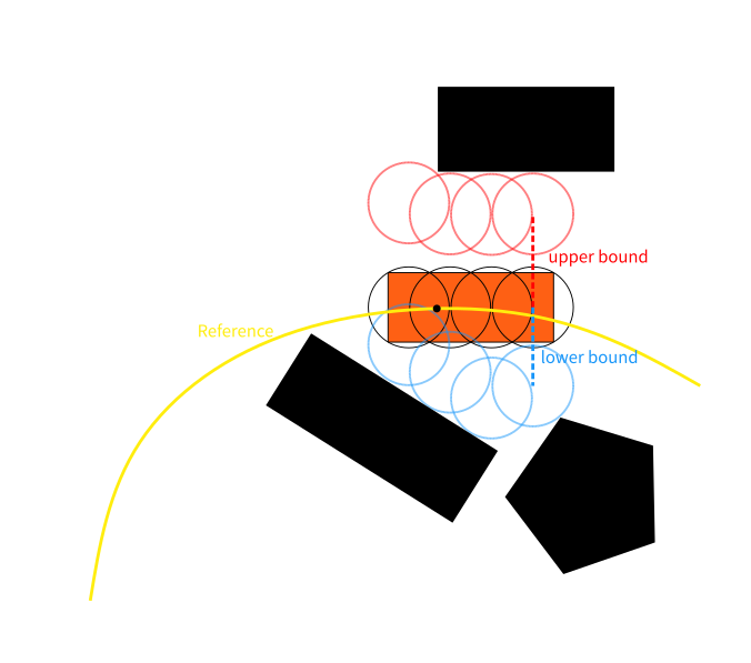
(1) Use four circles to represent the vehicle.
(2) Sample uniformly along the smoothed reference path to get n points, with a spacing of 0.3m. Each point will correspond to a vehicle state to form a path.
(3) For each point, assuming that the vehicle center (rear axle) coincides with that point, calculate the lower and upper bounds of the circles: .
is the offset of the k th circle at the i th point from the original position. These bounds will be used as constraints of the optimization later.
(4) Formulate QP.
The vehicle state in the Frenet frame is
. After the optimization, n vehicle states in the Frenet frame, corresponding to the n points on the reference path, are calculated to form a path.
State variables: z =
Control variables: u = (curvature's derivative w.r.t. the arc length s).
Dynamics constraints: According to Trajectory planning under vehicle dimension constraints using sequential linear programming III-A, the linearized and discretized system dynamics are .
Position and heading constraints: For every state on the result, the four circles representing the vehicle shape have to be within the bounds calculated above. So the connection between the vehicle states and the position of the circles are built:
. As stated before,
.
Soft constraints on safety margin: Apply soft constraints on one of the circles. Take the forth circle for example: .
is a fixed safety margin,
is the slack variable.
Curvature constraints: .
Initial state and target state constraints: .
Optional: Keep the control variables constant for some steps to accelerate the optimization. .
Cost function:
Solve it.


