Tutorial

This tutorial should only take a few minutes to complete and will guide you through the basics of how to use the TransPhyloMatlab software. All the commands of this tutorial are found in the file tutorial.m.

Step 1: simulate an outbreak

If you want to obtain exactly the same results as in this tutorial, you should start by initialising the random number generator to the same state as mine:

rand('state',0);randn('state',0);

To simulate an outbreak, use the command:

outbreak=simu(neg,popsize,beta,nu,ninf);

The parameters are as follows:

neg	Ne*g in years, ie the within-host effective population size (Ne) times generation duration (g)
popsize	the size of the population
beta	the infectiveness
nu	the rate of recovery
ninf	the number of infected hosts, or 0 for any number

For example:

outbreak=simu(100/365,1000,0.001,1,10);

Step 2: visualisation of the outbreak

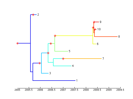
The outbreak object contains two interrelated components: a transmission tree and a phylogenetic tree. This can be visualised as a coloured tree using the following command:

plotBothTree(outbreak);

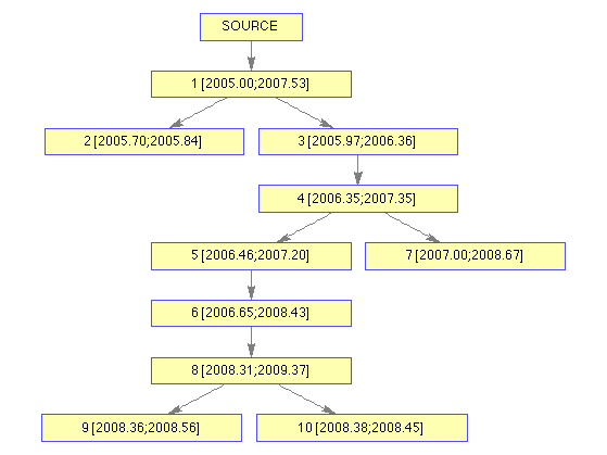
Or you may extract and plot just the transmission tree:

plotTTree(ttreeFromFullTree(outbreak));

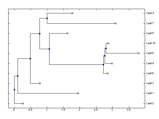
Or you may extract and plot just the phylogenetic tree:

plotPTree(ptreeFromFullTree(outbreak));

Step 3: inference of transmission tree given a phylogeny

We have previously simulated an outbreak containing both transmission tree and phylogeny. We now forget about the transmission tree, and try to re-infer it based only on the phylogeny. Let us start by extracting the phylogeny:

ptree=ptreeFromFullTree(outbreak);

To infer the transmission tree given this phylogeny we use:

timeLastSeq=max(outbreak(:,1));
result=infer(ptree,10000,timeLastSeq);

This will run the MCMC for 10,000 iterations, which takes approximately a minute on this example. The last argument timeLastSeq is the calendar date at which the last sequence was taken and is given in our simulated example by the first line. This is optional, but allows for the result to be dated absolutely (rather than relatively) since the phylogeny itself is in relative time. The result is a structure with 10,000 entries corresponding to the states of the MCMC.

Step 4: visualisation of the MCMC result

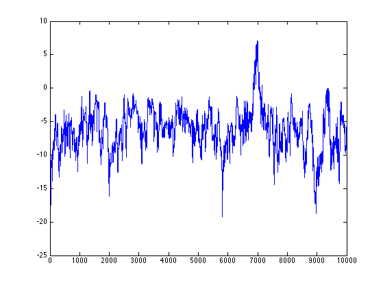
The log-prior and log-likelihood values are stored in the pTTree and pPTree members, respectively. To plot the trace of log(posterior)=log(prior)+log(likelihood) probability, we therefore use:

plot([result(:).pTTree]+[result(:).pPTree]);

To plot the trace of a parameter, for example beta:

plot([result(:).beta])

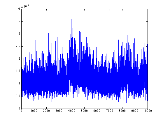
To plot the posterior distribution of probability to be the source case, based on the second half of the MCMC:

hist([result(end/2:end).source],1:10);

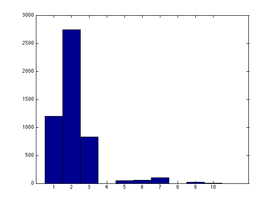
To plot the configuration after the first half of the MCMC:

plotBothTree(result(end/2).tree);

Step 5: beyond this tutorial

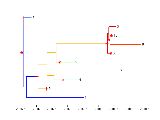
This tutorial provided an overview of how TransPhyloMatlab can be used on a simulated dataset. To apply to a real dataset, the phylogeny can be read from a Newick file using the command:

ptree=readPTree(filename);

The transmission tree can then be inferred as in step 4 above, using the command:

result=infer(ptree);

The key command infer is used to infer the transmission tree given a phylogeny using an MCMC. This function will probably need to be edited before it can be used in real-life situation, for example to specify a different starting point of the parameters (lines 9-12) or which MCMC moves should be used (lines 28-42).