Overview

Slicer Markups to Model is an extension of 3D Slicer for creating 3D surface models. The user first specifies a series of input control points, then the module creates a model from those points. Currently there are two types of surface models that can be created: closed surfaces and curves.

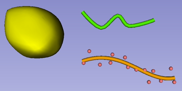
Example models created using SlicerMarkupsToModel. Left: Closed Surface. Right: Curves.

A simulated tumor is segmented on live ultrasound as a closed surface. Link

Curves are used to reconstruct catheter paths in a phantom. Link (See "Electromagnetically-generated catheter paths for breast brachytherapy")

GUI Features

The main GUI for this module

The parameter node is used to store all options settings for the module. The parameter node can also be saved along with a Slicer scene. When the scene is later re-opened, all options and settings should be preserved.

The two radio buttons along the top indicate whether the model should be a closed surface or a curve.

The Input Node is used to store input points for the model. There is an option to create a new Markups Point List from the drop-down selector. A Markups Point List can be added or deleted using buttons beside the selector. (*Note that advanced users can also take as input a "Model" and work with points from polygonal data).

The Output Model Node stores the model created by this module.

The Update Button can be set either to manual mode (updates only happen when the button is clicked), or to automatic mode (updates happen whenever the parameters are changed or when the input points are changed). Click on the checkbox to toggle between these two modes.

The Display Panel allows convenient access to change basic rendering properties of the model and input markups.

The Display Panel as seen in the GUI.

• Model Visibility: Toggle visibility in all views.

• Model Opacity: Change opacity. (Larger = more opaque)

• Model Color: Change the color of the model in all views.

• Model Slice Intersections: Toggle visibility in the red, yellow, and green slice views. Model Visibility (above) must also be enabled.

• Markups Text Scale: Change the size of text beside each input markup control point.

Closed Surfaces

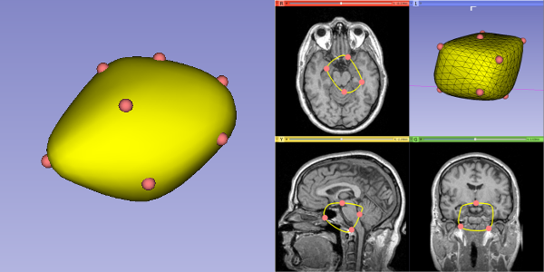
Left: Example of a closed surface. Right: Example of how a closed surface might look in slice view.

Closed surfaces are convex models that enclose the input points. Every time a new input point is added, the closed surface expands to contain the new input point. There are a variety of parameters that can be tweaked through the Closed Surface Model Settings panel.

Panel when working with a closed surface.

• Clean Duplicated Input Points: Remove duplicates from the input points

• Smoothing: Make the closed surface smoother by using the "Butterfly Subdivision". Note that sometimes concavities and self-intersections will occur after applying this smoothing. See "Force Convex Output" below.

• Convexity: Only tetrahedral 'cells' contained in a sphere with this radius will be used to construct the model. Concavities can be introduced by changing this value. (Note that 0.0 means that this feature is ignored, 0.0 is recommended for most applications.)

• Force Convex Output: The model will become fully convex after all other operations. Used to correct self-intersections introduced by butterfly subdivision.

Curves

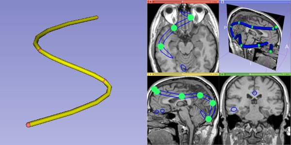
Left: Example of a curve. Right: Example of how a curve might look in slice view.

Curves are models shaped like a tube that either interpolate the input points, or approximate them in a best fit. There are in fact four types of curve in this module: Piecewise Linear, Cardinal Spline, Kochanek Spline, and Polynomial. All curves share the following parameters that can be seen on the Curve Model Settings panel.

Panel when working with a curve.

• Clean Duplicated Markups: Remove duplicates from the input points.

Piecewise linear curves are the simplest type of curve that can be created. A tube model is created that passes from one input point to the next in the original order specified from the point list.

Cardinal spline curves appear smooth. A tube model is created that passes through each input point in the order specified from the point list. Between each pair of points, there will be some curvature in the model. See Wikipedia to learn more about cardinal splines.

Kochanek spline curves appear smooth. A tube model is created that passes through each input point in the order specified from the point list. Between each pair of points, there will be some curvature in the model. See Wikipedia to learn more about Kochanek splines.

• Curve is a Loop: Indicate if the Curve should loop from the last point back to the first point (Valid for splines only).

There are a few paramters specific to Kochanek Splines, as seen in the Fitting panel.

Additional parameters shown on the Fitting panel for Kochanek splines.

• Ends copy nearest derivative: The first and last points should use the tangent from their nearest neighboring points.

• Kochanek Bias, Kochanek Tension, and Kochanek Continuity: As indicated on Wikipedia.

Global Least Squares Polynomial curves appear smooth. Unlike the other types of curve, polynomials approximate the input points instead of interpolating them. This particular option creates a global approximation to the data. The curve is represented using a tube-shaped model.

Moving Least Squares Polynomial curves appear smooth. Unlike the other types of curve, polynomials approximate the input points instead of interpolating them. This particular option creates a curve based on local approximations to the data. It's slower than the global least squares polynomial, but it tends to follow the data better. The curve is represented using a tube-shaped model.

There are a few parameters specific to Polynomial curves, as seen in the Fitting panel.

Additional parameters shown on the Fitting panel for polynomials.

• Point Sorting: This tells the module how to determine the order of the input points. If the input points are already in order, use "Indices". If the point order is unknown and the polynomial should connect the farthest two points, use "Minimum Spanning Tree".

• Polynomial Order: How closely the polynomial should follow the input points. (Larger = closer fit, but also increased risk of overfitting)

• Sampling Width: (Moving Least Squares Polynomial only) How much of the data should be used to create local polynomial fits. This is represented in normalized parameter space, meaning that 0.5 (for example) will capture half of the length of underlying data. (Larger = looser fit but more numerically stable, smaller is closer fit but higher risk of numerical instability and risk of overfitting)

• Weight Function: (Moving Least Squares Polynomial only) This tells the module how local polynomials should treat data that is farther away. Rectangular indicates that all data within the sampling width should be treated with equal importance in each fit (fast, but susceptible to noise and sudden turns in underlying data). The other options, Triangular, Cosine, and Gaussian, indicate that data should be treated less importantly if it is far away. Note that the Gaussian option uses a curve with three standard deviations (capturing 99.7% of the Gaussian curve area).

Under Tube Properties you can change certain aspects of the curve model's geometry (size, resolution).

• Radius: (Under Tube Properties) Changes the radius of the tube model (larger = wider tube).

• Number of Sides: (Under Tube Properties) Changes the outer smoothness of a tube model (larger = smoother appearance).

• Segments Per Point: (Under Tube Properties) Changes the number of points used to interpolate/approximate a curve. (larger = smoother appearance).

• Capping: (Under Tube Properties) Changes if the ends of the output tube should be capped.